Response Time SLA
Percentiles, histograms, and missed SLA counters
Response time (or latency) percentiles are a ubiquitous measure of system performance. The P999 (99.9th percentile) is a high bar, so it’s a good metric to determine an SLA. For example, my team runs a system with an 800 millisecond response time SLA determined by the P999. To meet that SLA, 99.9% of all requests must take <= 800ms. The system meets the SLA, but here’s its P999 graph:
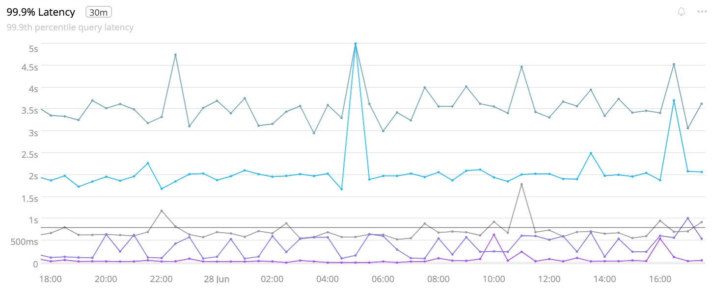
Looks bad, but the system is meeting the SLA. To understand why, let’s look at how percentiles are calculated. The Percentiles page on this site is a longer, more technical read about the subject, but for our purposes here the TL;DR is: a percentile is a high water mark. Consider a literal high water mark:

The line between the white and dark brown rock is the high water mark and analogous to the P999. It tells us only one thing: at least once, the water rose that high. That’s good to know, but going forward we’d really like to know: “How many times does the water rise that high? And, when it does, how long does it stay there?”
“Wait a minute,” you might be thinking, “that’s exactly what a percentile defines: how many.” That’s true, so for P999 you can multiple the number of queries in a period by 0.1% to calculate how many queries the percentile excludes. For example, with 10,000 queries, the P999 excludes the top 10 queries. So if the P999 = 2s, then approximately 10 queries were >2s.
Here’s the important point: percentiles are almost always a statistical calculation from a sample. (And there are several different calculations and sampling algorithms.) Sampling is required for fast, efficient metrics at scale. It works really well for calculating percentiles. From a sample of only 2,000 values, an accurate percentile can be calculated, so there’s no need to save and sort tens or hundreds of thousands of values per metric reporting period.
Histograms
We get accurate percentiles from samples, but samples clobber the true distribution of values. The same P999 value can be calculated from very different distributions. Here’s the proof for 100 values distributed in 100ms buckets:

In histogram 1, the vast majority of queries (98%) are fast: 200ms. Only 2 queries were 1500ms.

In histogram 2, the queries are split evenly between 50% fast (200ms) and 50% slow (1500ms).

In histogram 3, the queries are somewhat evenly distributed, a good number (but not a majority) are fast, and the are queries in every bucket up to 1500ms.
Percentiles are ubiquitous, but response time (or latency) distribution histogram are rare, which is unfortunately because they reveal the quality of response times. Histogram 1, despite its high P999, is great quality. We can ignore the rare times its slow. Histogram 2 is suspicious quality: sometimes fast, sometimes slow? That’s unusual and should be investigated. Imagine if half the time you commute to work it takes 20 minutes and the other half it takes 2.5 hours—that’s the same scale difference (7.5x). Histogram 3 is confusing quality: often fast, but 800ms to 1500s combined is significant. There might be an optimization to get the distribution back to something like histogram 1.
Percentile is quantity and distribution is quality. Histogram 2 illustrates this: even if P999 = 1500ms is acceptable, having 50% of queries be slow is unacceptable. It’s important to look at the distribution of values, but this isn’t easy because distributed histograms at scale are not common. Fortunately, there’s an easy measurement which serves the same purpose: a missed SLA counter.
Missed SLA Counter
A missed SLA counter counts the number of times something misses a predetermined SLA. As mentioned at the beginning of this post, our system has an 800ms response time SLA. When a request takes longer than 800ms, the SLA counter is incremented. The exact percentage of missed SLA responses equals:M = missed / total * 100.
The great thing about M: it doesn’t depend on percentiles, statistics, samples, or distributions. It’s exact and directly meaningful. If M <= 0.1, then 99.9% of responses met the SLA, regardless of the P999 or distribution. This is why our system meets the SLA despite having a high P999. As it turns out, M = 0.11 for the system, which means the distribution is like histogram 1: responses are almost always fast, but when they miss the SLA, they tend to miss it big (2-3.5s).
Distribution of Percentiles
Which P999 is the true high water mark? Most systems, like ours, are deployed to many app instances, each of which might perform differently. And a sharded back-end database affects response times, too.
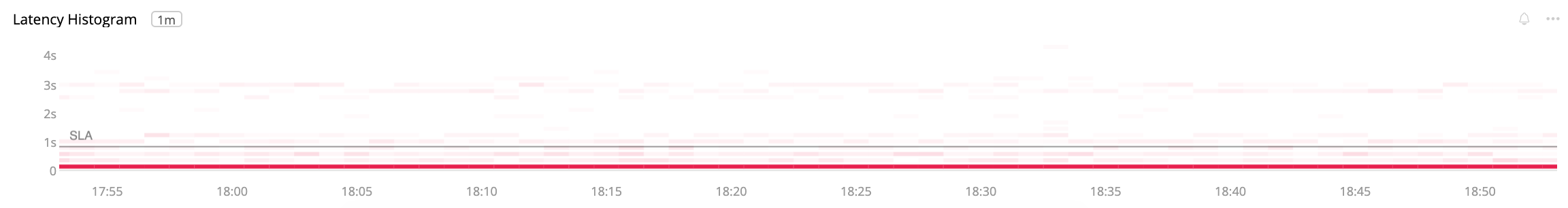
The chart above is a SignalFx histogram of P999 values from our system. The dark, solid red line at bottom shows that P999 values are most frequent around 200ms. Sometimes they float up to the SLA at 800ms, but overall P999 is below or around the SLA. This accords with M = 0.11 for the system.
Point is: percentiles fluctuate, too. We tend to write, talk, and think of the P999 (or any percentile) as one value, but it has a distribution, too. If all parts of the system are stable, the distribution of P999 should be very narrow, like histogram 1. The same quantity vs. quality consideration applies: if the distribution of a percentile is poor (i.e. widely distributed, having many disparate values), then some parts of the system aren’t performing as well as others. In fact, we see this in our system: on some app instances the P999 is 700ms, and on others it’s 3.5s. Not all hardware, cloud compute, databases, etc. perform equally well.