Percentiles

Percentiles are ubiquitous in application performance monitoring, particularly the 95th (P95), 99th (P99), and 99.9th (P999) percentiles. The basic concept is simple: percentile Pn means n% of all values are <= than the Pn value. If the P95 value = 100ms, then 95% of all values are <= 100ms. In other words: 5% of all values are > 100ms. Percentiles discard the top (100-n)% values as outliers for various reasons which are outside the scope of this page. Less simple than the basic concept is calculating percentiles, which is the scope of this page. Given arrays x and y with index j:

The percentile rank for each array element is given. For example, x[4] is P50 (median): <= x[4] is exactly half (50%) of all 10 values. Here’s where percentiles get interesting: where is P95? If x[8] = P90 and x[9] = p100 then P95 is between these element which does not exist (i.e. x[8.5] is not valid). Do we choose x[8] or x[9]? The answer depends on the method: nearest rank or linear interpolation.

First, a few definitions to make what follows easier to follow:

• p: Percentile as fraction: 0.90 for P90, 0.95 for P95, etc.
• i: i-th order statistic (explained below)
• j: i-1
• k: Integer part of i (if i=8.53 then k=8)
• f: Fractional part of i as integer (if i=8.53 then f=53)
• n: Number of values recorded (sample size)

In statistics, the “order statistics” is a sample of n observations ordered least to greatest (ascending): {X₁,…,X_n}. i is the i-th values: X_i. In code, we adjust for the zero-indexed array by subtracting 1 from i. To make the distinction clear, j is i adjusted.

Nearest Rank

For arrays of sorted values, the percentile rank at index j is math.Ceil(p*n) - 1. The base calculation is i = p * n.¹ Fractional i are not valid, so math.Ceil rounds up if i is not a whole number. And - 1 adjusts for the zero-indexed array, yielding j. The base calculation has variations,² but this is the simplest and often used in code because it can be used inline like: pval := values[int(math.Ceil(p*n))-1]. The most important point is:

• Fractional i must be rounded up

In Go this could be wrong for P95: values[int(n*0.95)-1]. For n=10, the result is int(9.95) which Go truncates to 9. It should be rounded up to 10. The importance of rounding up becomes more clear with an array like []y.

Except for P100, []y has no whole number percentiles at any rank. The P90 rank in []y is i = 0.90 * 11 = 9.9, which is j = i - 1 = 8.8. This is when rounding up is important: y[8] is P81.82 which is far from P90, but y[9] is P90.91 which is very close—y[9] is the nearest rank for P90.

Nearest rank works best with at least n=1000, else P99 and P999 are the top two values which defeats the purpose of percentiles: to discard the top (100-n)% values.

Software can quickly and easily record thousands of values, creating a representative sample for which the nearest rank calculation works very well. But physical systems and humans are usually a little slower and time-consuming, perhaps only able to record tens or hundreds of values. When the sample size is relatively small, linear interpolation is a better method for calculating percentiles.

Linear Interpolation

Linear interpolation estimates the value between two ranks. If you Google it, you will find that different programs (Microsoft Excel, MATLAB, etc.) use slightly different equations. Wikipedia has three variants, but the primary source is Sample Quantiles in Statistical Packages by Rob J. Hyndman and Yanan Fan. The TL;DR is the equation on page 363 (page 4 of the PDF),

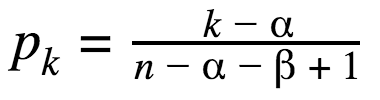
and Table 3 on the next page which lists values for the constants, and section “5. SUMMARY AND CONCLUSIONS” which concludes that “[definition 8] is the best choice.” Definition 8 is more commonly called “R8”.³ R6 and R7 are good choices, too, so R6, R7, and R8 are commonly used in software.

Implementing linear interpolation has two steps. The first is calculating i with one of the R-equations. Unlike nearest rank, i is not rounded or adjusted for the zero-indexed array. Instead, its fractional and integer parts are used in the second step. The common R-equations for linear interpolation implemented in Go:

i := p * (n + 1)                 // R6
i := p * (n - 1) + 1             // R7
i := p * (n + (1/3.0)) + (1/3.0) // R8

Those lines of code are the equation solved for k. For R6, α=0 and β=0 which simplifies to p_k=k/n+1, then k=p_k(n +1) which is the first line of code (where k = i).

The second step interpolates the percentile value by adding the lower rank value to the diff of the upper and lower rank values multiplied by f, the fractional part of i. Let’s put it all together in Go code that demonstrates using R6, R7, and R8 with known input and output values for P90:⁴

package main

import (
	"fmt"
	"math"
	"sort"
)

// https://www.itl.nist.gov/div898/handbook/prc/section2/prc262.htm
var control = []float64{95.1772, 95.1567, 95.1937, 95.1959, 95.1442, 95.0610, 95.1591, 95.1195, 95.1065, 95.0925, 95.1990, 95.1682}

func main() {
    sort.Float64s(control)
    N := float64(len(control))
    p := 0.90

    iR6 := p * (N + 1)
    fmt.Printf("R6: %.4f\n", pValue(iR6, control))

    iR7 := p*(N-1) + 1
    fmt.Printf("R6: %.4f\n", pValue(iR7, control))

    iR8 := p*(N+(1/3.0)) + (1 / 3.0)
    fmt.Printf("R8: %.4f\n", pValue(iR8, control))
}

func pValue(i float64, vals []float64) float64 {
    k, f := math.Modf(i)           // 8.53 -> k=8, d=53
    lower := vals[int(k)-1]        // vals[7]
    upper := vals[int(k)]          // vals[8]
    return lower + f*(upper-lower) // vals[7] + 0.53 * (vals[8]-vals[7])
}

Function pValue is the second step of the equation which differs only by the R-calculated i. k, the integer part of i, is the lower boundary when subtracted by one to adjust for the zero-indexed array. k is also the upper boundary when not adjusted for the zero-indexed array. Then add and multiple the upper and lower boundary values with f, the fractional part of i, as shown. The result is an interpolated P90 value. The value is somewhere between the upper and lower rank values. Whereas nearest rank yields an observed value that might not be the actual percentile, linear interpolation yields a non-observed value that is statistically equivalent to the actual percentile.

Let’s go back to the original question—where is P95?—with []y. The i for each R-equation is:

• R6: i = 11.4
• R7: i = 10.5
• R8: i = 11.1

Since those are non-adjusted lower boundary i, R6 and R8 do not work because y[10] is the maximum value. But R7 would return a value between y[9] and y[10]. By contrast, nearest rank returns the value at y[10]. For this small sample, R7 is the most accurate because P95 is, by definition, less than the maximum: P95 < P100.

Comparison

P999 request latency (response time) is the gold standard for high-performance, low-latency applications. To determine which methods is most accurate for P999, I compared nearest rank, R6, R8, and “Hybrid R6/7/8”.

For nearest rank, the values are not sampled. This is the simplest, most basic approach but not commonly used because it is not memory-bounded. For example, file “100k-1-or-2” has 100,000 values. For 8-byte float64 values, one sample is 800K. Not terrible but also not necessary because, as that line shows, all the algorithms are very close to the real P999 value highlighted green. (Real values in green arise when the P999 rank happens to be a whole number.)

For R-equations, the sample size 2,000 using “Algorithm R” by Jeffrey Vitter (random uniform sample). Hybrid R8 (4k) is the exception: sample size 4,000.

R6 and R8 (2k) use their respective R-equations, but “Hybrid R6/7/8” use both methods: nearest rank if the sample is full (n >= 2000), else the respective R-equation. The reason for “hybrid” algorithms is discussed later. First, let’s look at the results (click to open PDF):

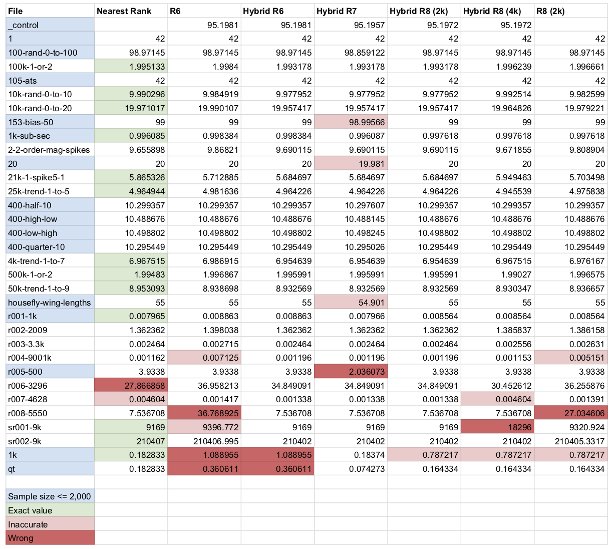
Hybrid R8 (2k) is the clear winner: only one inaccurate value for file “1k”. File “r008-5550” demonstrates the benefit of the hybrid algorithm: R6 and R8 (2k) are wrong, but all the hybrids are accurate. Files “1k” and “qt” demonstrate why R8 is the best: R6 is wrong, and R7 is best for “1k” but wrong and inaccurate for other cases. Overall, the data agrees with what Hyndman and Fan concluded: R8 is the best choice. Even better: Hybrid R8, which is what go-metrics uses.